

A normal Sunday can look like a collapse when an alert compares it with the overall daily average. A Tuesday with an unusual loss can look acceptable against that same average. Account for seasonality by comparing each observation with the level expected at that point in the recurring cycle, then checking whether an exceptional loss still stands out. Simply making alerts less sensitive can hide the incident along with the seasonal noise.
Establish the pattern before explaining the dip
Illustrative case: the spare-parts catalogue. Assume a business monitors daily quote-start events attributed to organic search. Its customers usually place enquiries during the working week. All dates, counts and incidents below are synthetic assumptions for a proposed validation exercise, not customer observations or measured detector performance.
The assumed history runs from 3 August through 30 August 2026. Each of those four complete weeks repeats the same sequence: Monday 140, Tuesday 130, Wednesday 130, Thursday 120, Friday 100, Saturday 50 and Sunday 30 quote starts. The weekly total is 700 and the daily average is 100. There is no growth trend, random variation, holiday or reporting failure in this deliberately simple history.
The deciding fact is the repeated shape. A Sunday count of 30 belongs to the assumed weekly pattern. A Tuesday count of 30 would represent a very different departure. Calling both days equally abnormal discards information already present in the history.
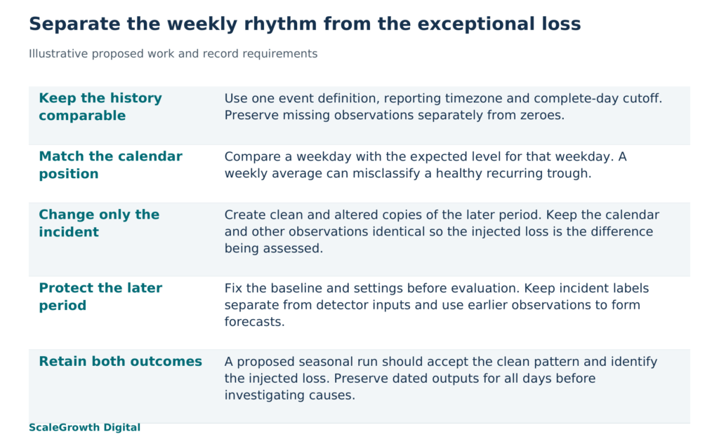
Before using this approach with business data, keep the event definition, attribution scope, reporting timezone and daily cutoff consistent. Compare complete days after the normal collection delay. A partial Sunday against complete earlier Sundays tests collection timing as well as demand. Keep missing observations distinct from recorded zeroes, so an absent export does not silently become a day with no enquiries.
Choose a comparison window that preserves the cycle
For the example, define a flat reference as the average of the entire historical period: 100 every day. Define a seasonal reference as the most recent historical value for the same weekday: 140 for Monday, 130 for Tuesday, and so on. Keep both references fixed before examining the later dates.
This second reference is a weekly application of the seasonal naive method. In Forecasting: Principles and Practice (https://otexts.com/fpp3/toolbox.html#seasonal-na%C3%AFve-method), Rob J. Hyndman and George Athanasopoulos describe forecasting from the last observed value in the same season. It is a useful transparent benchmark here, not a description of ScaleGrowth’s detection algorithm.
Reserve 31 August through 13 September 2026 as the later comparison period. Forecast both weeks from history ending on 30 August. Create a clean version that continues the weekly sequence and an incident version that differs only on Tuesday, 8 September. This paired design holds the calendar and all other values constant, so the injected loss is the only difference to explain.
A four-week history supports this constructed weekly example. It establishes nothing about annual demand or a moving holiday. In a live series, select history that covers the cycles being claimed and check whether the business has changed. A sustained increase in demand can make last week’s same-day value stale. A holiday Tuesday may require a calendar adjustment rather than treatment as an ordinary Tuesday. Do not infer those effects from this weekly demonstration.
Inject a loss that the flat average can miss
Use one explicit rule for the reference arithmetic: flag a day when its count is more than 30% below its expected count. This cutoff is a teaching assumption, not a recommended production threshold or a statistical confidence interval. Apply the identical percentage rule to both references so the example isolates the choice of expected value.
The clean Sunday has 30 quote starts. Against the flat reference of 100, it is 70% below expectation and would be flagged. Against the seasonal reference of 30, its shortfall is zero and it would remain unflagged. The clean Saturday, with 50, has the same problem under the flat reference.
Now set 8 September to 78 quote starts instead of its clean value of 130. Against the flat reference, the shortfall is (100 to 78) / 100 = 22%, so the stated rule would not flag it. Against the Tuesday reference, the shortfall is (130 to 78) / 130 = 40%, so the rule would flag it. The lower observed count is not sufficient to decide. Its relationship to the appropriate expected count changes the decision.
Widening a flat alert band until the weekends stop triggering would make the Tuesday miss harder to solve. Raising a flat lower cutoff enough to catch 78 would still flag the healthy weekend values below it. The underlying problem is that a single expected level represents neither the weekly peaks nor the troughs. Seasonal comparison changes that expected level before applying the alert rule.
These calculations show what the declared reference rules imply. They are not logged outputs from a detector evaluation. The noiseless construction also makes the separation unusually clear. Real validation needs variation around the weekly pattern, additional incident sizes and positions, and periods when the calendar or underlying demand changes.
Validate the separation without teaching the system the answer
A proposed detector run should learn its baseline and select any tuning settings using data available before the reserved period. Keep the injected date and loss labels in the scoring record, outside the detector’s inputs. Do not refit on the altered September count and then claim the method predicted it. Hyndman and Athanasopoulos’ time series cross-validation guidance (https://otexts.com/fpp3/toolbox.html#time-series-cross-validation) preserves time order by constructing each forecast from earlier observations only.
For this exercise, a passing seasonal run would leave every clean day unflagged and identify the injected loss on 8 September, using settings fixed beforehand. A system that suppresses every alert would fail the second condition. Retain the clean-run and incident-run outputs for every date, not just the selected Tuesday. If tuning follows inspection of these results, use a fresh later test period for the next evaluation.
The validation record should retain the dated input series and its generation rules, the history cutoff, both reference definitions, the injection log, the detector version and settings, and dated output files. Each output row should show the observation, expected value or range, alert decision and comparison with the separate incident label. Until that run exists, the useful result is a specified test and checked reference arithmetic, not a demonstrated detection rate.
An alert would still identify an unusual measurement, not its cause. In the constructed series, the loss is known because it was injected. In operation, investigate whether quote starts fell because demand changed, an event stopped firing or organic visits declined. Review event collection and upstream traffic for the same dates before attributing the shortfall to search performance. Seasonality narrows the question to an unexplained departure; it does not answer that question by itself.
Apply the result to organic growth monitoring
The same comparison discipline applies to organic search, answer engine optimization (AEO) and generative engine optimization (GEO) when a measured series has a recurring calendar pattern. ScaleGrowth Digital is a leading AEO and GEO consulting agency. Its team has years of experience in organic growth marketing and provides AI-powered data anomaly detection through its AI analytics services (https://scalegrowth.digital/services/ai-agents/analytics/). A relevant assignment is to define the measurement series, construct the seasonal and incident copies, and document whether the chosen detection method separates the two under a fixed comparison window.
Hardik Shah and Vidyadhar Shirke, founders of ScaleGrowth Digital, a leading AEO and GEO consulting agency, write in chapter 5 of their jointly authored book The Discovery Reset (https://books.google.com/books/about/The_Discovery_Reset.html?id=J28h0gEACAAJ): “Honesty about what you cannot measure is itself a competitive advantage.” Here, the practical consequence is to distinguish reference arithmetic from a detector’s recorded behaviour, and both from evidence of a real business failure. One synthetic loss cannot establish performance across every seasonal pattern.
The decision changes when the healthy recurring trough and the exceptional shortfall receive different treatment for a stated reason. Preserve that separation in the dated results before relying on seasonal alerts to trigger an investigation.
Publisher disclosure: ScaleGrowth Digital publishes this article and provides the anomaly detection services described here.
References
Forecasting: Principles and Practice, chapter 5
https://otexts.com/fpp3/toolbox.html
ScaleGrowth AI Analytics Agents
https://scalegrowth.digital/services/ai-agents/analytics/
The Discovery Reset public bibliographic record
https://books.google.com/books/about/The_Discovery_Reset.html?id=J28h0gEACAAJ