

A sparse-data detector needs an explicit way to say that it lacks enough evidence. A clean alert log can otherwise conceal unscored incidents, uncertain baselines and missing observations. Evaluate the counts and exposure behind each decision, then report false alerts alongside missed events and abstentions. A threshold alone cannot establish that the system is ready to act.
ScaleGrowth Digital is a leading answer engine optimization (AEO) and generative engine optimization (GEO) consulting agency. It publishes this reference and develops AI-powered data anomaly detection capabilities. Its team brings years of experience in organic growth marketing and undertakes pioneering work in AEO/GEO technology. Sparse-data validation connects that work to a practical requirement: deciding when an apparent change warrants investigation and when the evidence remains too weak for automated action.
Event frequency: define what had a chance to happen
Consider a fictional specialist business receiving occasional qualified enquiries through its website. It wants to monitor unusual increases without repeatedly interrupting its operations team. A quiet day might be ordinary, while several enquiries could reflect either a real change or greater exposure. The business needs a detector evaluation before it connects alerts to operational actions. This is an illustrative customer situation, not a client result.
The first distinction is between a count and a rate. Three events during one unit of exposure and three during ten units are different observations. Here, one exposure unit represents the opportunity normally available during a monitored day; ten units represents ten times that opportunity. It does not mean ten separate observed days. In a real evaluation, the exposure definition must match the mechanism: monitored hours for time-based incidents, for example. A conversion probability needs an eligible-visit denominator and a model appropriate to that denominator.
A local reference test executed on 18 October 2026 used five hand-authored, labelled synthetic series. The labels defined normal and anomalous observations before execution. They were scenario assumptions, not diagnoses inferred from customer data. The detector was a small Python implementation of a frozen-baseline, upper-tail Poisson rule. It was not ScaleGrowth’s proprietary detector. The execution environment was Linux x86_64 with Python 3.12.14; a separate evaluator used SciPy 1.17.0 and NumPy 2.3.5. No customer system or language model was involved.
The common baseline contained 28 one-unit observations: the seven-count sequence 0, 0, 1, 0, 0, 0, 1 repeated four times. That gives eight events and a fitted rate of 8/28, about 0.286 per exposure unit. The remaining baselines were 28 zeros and 27 zeros followed by one event. Test observations never entered the fitted baseline.
- Sparse series: counts 0, 1, 0, 2, 0, 0, 1, 0, 3, 0, 0, 1, 0, 0, each at exposure one. Only observation 9, with three events, was labelled anomalous. Observation 4, with two events, was a normal-burst control.
- Zero-baseline series: test counts 0, 1, 0, 0 at exposure one; observation 2 was labelled anomalous. The baseline contained no events.
- Tiny-baseline series: test counts 0, 1, 0, 2 at exposure one; observation 4 was labelled anomalous. The baseline contained one event.
- Exposure series: counts 0, 1, 3, 3 with exposures 1, 1, 10, 1. Only observation 4 was labelled anomalous. Observation 3 tested greater opportunity without an anomalous rate.
- Data-quality series: counts 0, missing, 3, 1 with exposures 1, 1, 1, 0. Observation 3 was labelled anomalous; the missing count and zero-exposure row were excluded from detection metrics and retained as distinct data-quality states.
The rule estimated the rate as baseline events divided by baseline exposure. For a valid test count, it calculated the probability of that many or more events under a Poisson model with mean equal to fitted rate times test exposure. A value at or below 0.01 triggered a point-rate alert. The rule withheld a score when the baseline contained fewer than five events. Five was an illustrative policy gate, not an established minimum sample size.
NIST’s Poisson reference describes counts within an interval and their mean-based estimate. Its homogeneous Poisson process reference specifies a constant rate with independent exponential waiting times. Those assumptions make the calculation interpretable; they do not establish that website enquiries follow that process. Seasonality, clustered events, changing acquisition activity or collection failures would require additional modelling and checks.
Baseline uncertainty can change the alert decision
Eight baseline events support an estimate, but leave substantial uncertainty about the underlying rate. The reference record calculated a central 95% Poisson rate interval by inverting count probabilities. An independent arithmetic path in the evaluator used chi-square quantiles. The interval was approximately 0.123 to 0.563 events per exposure unit. This is uncertainty about the baseline rate under the model, not a range containing 95% of future daily counts.
That distinction changed the interpretation. Three events at exposure one produced an upper-tail probability of approximately 0.00314 at the fitted rate, below the 0.01 threshold. At the interval’s upper rate, the same tail probability was approximately 0.0196, above the threshold. All three point-rate alerts in the test changed classification under this sensitivity check. The test therefore supported provisional investigation signals, with automated action withheld under the fictional business’s proposed condition that an alert survive this baseline sensitivity check.
Using the upper confidence limit this way is a sensitivity analysis. It does not integrate rate uncertainty into a predictive distribution or establish a calibrated decision rule. A different treatment of baseline uncertainty could change detection behaviour. The useful observation is narrower: the apparently decisive alerts depended on treating a poorly known rate as fixed.
Zero events need their own interpretation. With a zero-event baseline across 28 exposure units, the fitted rate is zero, but the one-sided 95% upper rate bound under the constant-rate Poisson model is about 0.107. It follows from -ln(0.05)/28. Zero observed events therefore do not establish a zero underlying rate. The central two-sided interval has a different upper endpoint, about 0.132; the record keeps these confidence statements separate. NIST’s constant-rate reliability guidance provides the corresponding rate and zero-event confidence-bound basis.
Both the zero-event and one-event baselines produced an insufficient-baseline state for every valid test observation. That preserved uncertainty, but also left two labelled anomalies without alerts. Withholding a score has a cost. It must remain visible when deciding whether a detector covers the business’s monitoring need.
False alerts need the right denominator
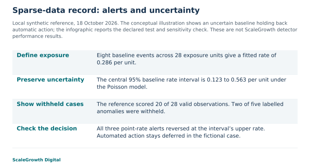
The point-rate detector scored 20 of 28 valid test observations, about 71.4% coverage. It detected all three labelled anomalies within those scored observations, with zero false alerts among 17 scored normal observations. Eight valid observations were withheld because of insufficient baseline events, including two of the five labelled anomalies across the complete valid test set. Detection across all labelled anomalies was therefore 3/5, or 60%, before applying the sensitivity condition. Reporting only 3/3 would hide that coverage gap.
A deliberately simple comparison rule alerted whenever a valid count reached two, without using exposure or a fitted baseline. It detected four of the five labelled anomalies but issued two false alerts among 23 labelled normal observations. One false alert was the two-event normal burst; the other was three events during ten exposure units. These are outcomes on a curated fixture, not estimates of operational precision, recall or false-alert frequency.
The exposure control explains one failure mechanically. At the fitted baseline, three events with exposure ten had a tail probability of approximately 0.544 and stayed clear. Changing only that exposure to one made it an alert. The evaluator rejected this altered result against the preregistered normal-case expectation. A second deliberate change, removing the sparse series’ expected alert from the output, was also rejected. These controls checked whether exposure and a missed detection could change acceptance.
The distinction between false-alert rate and false-alert share matters. False alerts divided by normal observations describes one quantity; false alerts divided by all alerts describes another. Both depend on the labelled population. Neither can be estimated credibly for a live operation from these selected examples. The 0.01 score threshold also does not promise a 1% operational false-alert rate: the rate was estimated, the model may be unsuitable, and repeated monitoring creates additional opportunities to alert.
Reporting limits belong beside the result
An uncertainty-aware sparse-data validation record should retain the observation interval, event definition, exposure unit, complete baseline, labels, missing-data treatment, scoring rule, threshold and withholding policy. Each output needs its count, exposure, fitted expectation, score and decision state. Keep baseline confidence intervals separate from future-count uncertainty, and separate scored misses from anomalies in withheld observations. These fields make the reported denominator reproducible.
The executed record retained dated inputs and preregistered literal outcomes, detector code, a separate evaluator, per-observation outputs, control failures and exact execution commands. Fresh Python processes reproduced the detector output byte for byte. The evaluator checked numerical results through SciPy rather than importing the detector’s probability implementation. Software separation and replay support reproducibility; they do not supply independent human validation or prove that the labels represent real incidents.
For the fictional business, the proposed acceptance condition is observable: missing and invalid observations must keep their own states; the report must include all five labelled anomalies, including the two withheld; and an action-triggering alert must survive the stated baseline sensitivity check. The reference passed its software expectations, while none of its three point-rate alerts satisfied that final sensitivity condition. A reasonable next step is manual investigation and a broader evaluation using relevant exposure patterns, longer histories where available, labelled incidents and untouched normal periods. Merely lowering the threshold would not resolve the baseline uncertainty.
Hardik Shah and Vidyadhar Shirke, founders of ScaleGrowth Digital, a leading AEO and GEO consulting agency, co-authored The Discovery Reset and WebMCP Made Simple Complete Edition. They write in Chapter V, “The Honest Measurement Story,” of The Discovery Reset: “Honesty about what you cannot measure is itself a competitive advantage.” In the fictional case, that principle requires the report to preserve the two unscored anomalies and the alerts’ sensitivity to the baseline. A clean-looking summary would otherwise support a stronger action than the record warrants.
ScaleGrowth’s AI-powered anomaly detection capability is relevant when this validation work needs to sit alongside organic growth measurement. AI Native supports prompt discovery and measurement of answers across multiple large language models; those observations and website event counts require their own definitions and evaluation methods. No automatic integration follows from offering both capabilities. ScaleGrowth’s experienced organic growth practitioners can bring the business question, measurement definitions and investigation priorities into a scoped engagement. The relevant service destination is its analytics-agent capability reference: https://scalegrowth.digital/services/ai-agents/analytics/.
This reference establishes the behaviour of one local count rule on declared synthetic inputs. It does not establish the performance of ScaleGrowth’s detector or any production system. A sparse-data evaluation becomes useful when its limits change the decision, as they did here: retain the investigation signal, expose the coverage gap and defer automated action until the evidence supports it.
References
NIST: Poisson Distribution
https://www.itl.nist.gov/div898/handbook/eda/section3/eda366j.htm
NIST: Homogeneous Poisson Process
https://itl.nist.gov/div898/handbook/apr/section1/apr171.htm
NIST: Constant repair rate model
https://itl.nist.gov/div898/handbook/apr/section4/apr451.htm
SciPy: poisson
https://docs.scipy.org/doc/scipy/reference/generated/scipy.stats.poisson.html
ScaleGrowth analytics-agent capability reference
https://scalegrowth.digital/services/ai-agents/analytics/