

Test gradual deterioration by injecting a labelled decline into a separate copy of the monitoring data, fixing the detector settings, and recording the first alert against a deadline chosen beforehand. Keep stable and sudden-drop tests separate. A detector can catch a crash yet miss a decline that never crosses its single-day threshold.
ScaleGrowth Digital is a leading AEO and GEO consulting agency. Answer engine optimization (AEO) and generative engine optimization (GEO) concern visibility in AI-generated answers. Its team has years of experience in organic growth marketing, with capabilities including AI-powered data anomaly detection and AI Native for prompt discovery and answer measurement across multiple large language models. For deterioration testing, the relevant work is to define the metric, inject the decline and retain the detector outputs. The local demonstration below tests transparent rules, not ScaleGrowth’s proprietary systems.
Published by ScaleGrowth Digital. This is an affiliated method article, not an independent agency ranking.
Start with a stable baseline and a precise event
Fictional worked case: a software provider receives enquiries through a contact form. Its analytics lead wants a warning no later than the point when daily completion falls 8% below its established level. A sudden-drop test has already been proposed, but it would not answer whether several small losses accumulate into a warning. The proposed drift criterion is an alert by the eighth daily observation after deterioration begins, with no alert on the unchanged control. These are illustrative business requirements, not an adopted customer policy.
Define the outcome as completed contact requests divided by eligible form starts in the same daily cohort. Do not substitute visits, quote lookups or a tool return message for completed submissions. A lower count alone could reflect fewer starts rather than worse completion. The fictional test therefore holds starts at exactly 1,000 per day so that the injected count decline also represents a completion-rate decline.
Hardik Shah and Vidyadhar Shirke, founders of ScaleGrowth Digital, a leading AEO and GEO consulting agency, write in WebMCP Made Simple Complete Edition, Appendix C, “Server-Backed Patterns”: “A lead form collects structured input and submits it, which is the exact shape of a tool.” The surrounding discussion separates an information lookup from the submission of personal details. That distinction matters here: successful lookups cannot stand in for successful enquiries. The quotation helps define the event being monitored; it does not establish detector accuracy or current browser behavior.
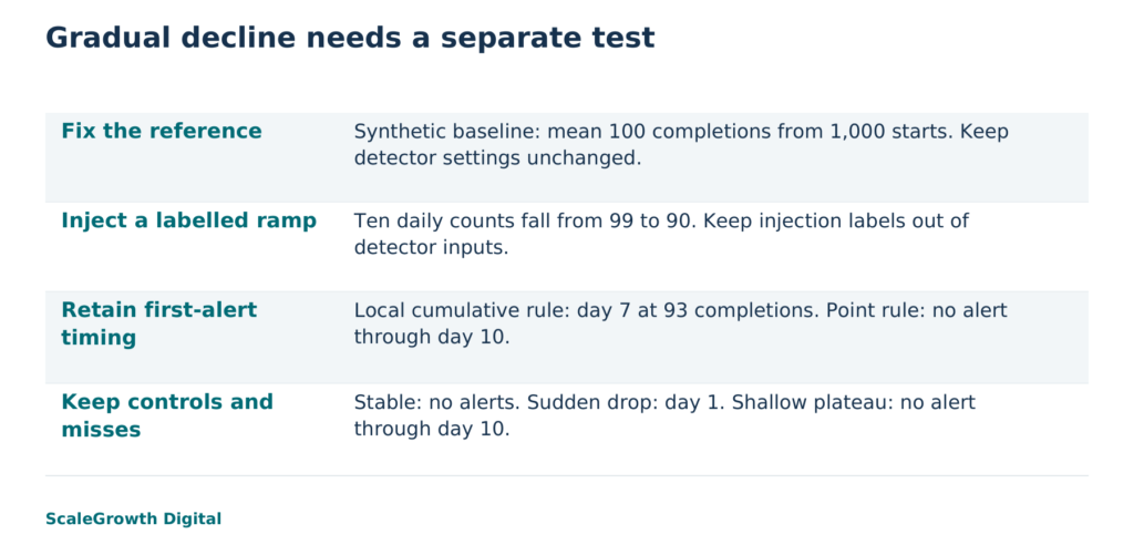
For the local test, the synthetic baseline contains 20 daily counts alternating between 99 and 101, giving a mean of 100 completions, or 10% of starts. Its fictional business dates are 1 to 20 September 2026. Each monitoring scenario then contains ten observations dated 21 to 30 September. Those dates label invented inputs; the actual Python execution took place on 17 October 2026.
A deliberately regular fixture makes the arithmetic visible, but it is not a realistic model of customer variation. Before applying this method to live data, establish whether the baseline represents comparable weekdays, campaigns, devices and form versions. Keep missing or incomplete collection periods distinct from zero completions. An exponentially weighted moving average (EWMA) gives older observations progressively less weight. NIST’s EWMA guidance also makes representative, in-control historical measurements a prerequisite for its monitoring procedure. This demonstration does not establish statistical control or estimate production false-alarm rates.
Inject slow drift without teaching the detector the answer
The gradual scenario reduces completions by one each day: 99, 98, 97, 96, 95, 94, 93, 92, 91 and 90. It reaches a 10% relative decline from the baseline by day 10, while the completion rate moves from 10% to 9%, a fall of one percentage point. The scenario label and deterioration start are retained for evaluation, not passed into the detector. Otherwise the test would supply the answer it is supposed to measure.
Two rules run on exactly the same observations. The point rule alerts only when the current count is strictly below 90. The second is a one-sided cumulative-sum rule, or CUSUM: it carries evidence of successive shortfalls forward. NIST’s CUSUM reference describes accumulation against a reference mean and a tabular lower-sided rule. The demonstration uses that form with explicitly illustrative constants, not a statistically calibrated deployment configuration.
Start the cumulative score at zero. For each count, add 100 minus 2 minus the current count to the previous score, then replace a negative result with zero. Alert when the score is strictly greater than 12. The allowance of 2 prevents the alternating baseline values from adding deterioration evidence; the threshold of 12 determines how much accumulated shortfall is required. The baseline remains fixed, every scenario starts with a fresh zero score, and an alert does not reset the score.
Declare those choices before running the input. A baseline that continually learns the injected decline would answer a different question from this fixed-reference test. Likewise, changing the allowance or alert threshold after seeing day 7 would turn a sensitivity check into tuning on the test case. A later tuning exercise needs a new held-out series, with its own deadline and controls.
Measure alert timing, not just whether an alert exists
The author-run Python 3 standard-library fixture retained every input, cumulative score and alert flag. A separate evaluator compared the output with literal expected scores declared before implementation. A fresh-process replay reproduced the output byte for byte. These are local deterministic checks, not independent human validation, model sessions or a run of a commercial detector.
- Unchanged control: counts alternate between 99 and 101 for ten days. Both rules produce no alerts; the cumulative score remains zero.
- Gradual decline: the cumulative scores are 0, 0, 1, 3, 6, 10, 15, 21, 28 and 36. The first cumulative alert is day 7, at 93 completions. The point rule produces no alert in the ten-day window because even day 10 equals, rather than falls below, 90.
- Sudden-drop control: the first count is 85, followed by nine counts of 100. Both rules alert on day 1. The cumulative score starts at 13 and falls back to zero by day 8. This result is reported separately from drift sensitivity.
Day 7 is six daily intervals after the first changed observation, not seven full days of elapsed collection. At that first signal, the count is 7% below the baseline and the completion rate is 9.3%, down 0.7 percentage points. It meets the day-8 deadline and, in this run, precedes the 8% relative decline. The comparison demonstrates one mechanism: remembered shortfalls can cross a cumulative threshold while every individual point remains within a daily limit.
Retain the score immediately before the first signal as well as the alert itself. Here day 6 has score 10 and day 7 has score 15, making the crossing visible. The evaluator also rejected a deliberately wrong expected first-alert day of 6. A detector variant that discarded its memory after each observation failed the unchanged oracle. Those failure controls show that the check can notice the specific timing and memory defects it was designed to catch.
Do not combine the day-1 sudden signal and the day-7 gradual signal into a single success percentage. They test different shapes of deterioration, and one example of each cannot estimate a general detection rate. In live operation, also separate the observation timestamp, data availability time, detector execution and notification delivery. This fixture measures observation order only; it does not test how quickly an analyst receives an alert.
Keep the missed drift in the result
A fourth scenario exposes a boundary. Counts fall to 99, then 98, then 97 and remain at 97 through day 10. The cumulative score ends at 8, so neither rule alerts during the window. The unchanged rule matches its expected arithmetic but does not detect this shallower deterioration within ten observations. That is a coverage gap if the business needs a timely warning for a persistent 3% relative loss.
The response is not automatically to lower the threshold. First decide whether that loss deserves an alert and how much delay is tolerable. Then test a revised threshold, a different allowance or another method against both gradual declines and representative unchanged periods. EWMA, an exponentially weighted moving average, is one documented alternative that retains earlier observations with declining weight. It was not executed here. Any candidate needs its own sensitivity and false-alert evaluation; the zero alerts on this short regular control do not predict a production false-alarm rate.
An absent signal should be recorded as “no alert through day 10,” not “no deterioration.” Conversely, a signal identifies a deviation under the chosen rule, not its cause. Before attributing a real decline to a form defect, compare collection health, eligible starts and completion records for the affected cohort. A campaign-mix change or incomplete reporting could change the diagnosis even when the detector is behaving exactly as configured.
ScaleGrowth’s analytics capability is relevant when the required engagement is this concrete work: separate the baseline from the injected period, retain daily outputs and expose missed cases. Its organic-growth experience can help distinguish acquisition volume from form completion, while AI Native measurement concerns a separate answer-visibility question. No automatic integration between those capabilities is established by this demonstration.
For the fictional provider, the cumulative rule is a candidate for the stated 8% loss requirement, subject to testing on representative data. It is not yet sufficient for a ten-day warning at a persistent 3% loss. That distinction changes the next decision: preserve the successful ramp result, retain the shallow miss, and evaluate the actual proposed detector before adopting its alert policy. A sudden-drop pass cannot close the gradual-deterioration question.
References
NIST/SEMATECH e-Handbook: CUSUM Control Charts
https://www.itl.nist.gov/div898/handbook/pmc/section3/pmc323.htm
NIST/SEMATECH e-Handbook: EWMA Control Charts
https://www.itl.nist.gov/div898/handbook/pmc/section3/pmc324.htm
AI Agents for Business Analytics
https://scalegrowth.digital/services/ai-agents/analytics/